mxxhcm's blog

  • 首页

  • 标签

  • 分类

  • 归档

Policy Distillation

发表于 2019-10-13 | 更新于 2019-12-17 | 分类于 强化学习

简介

Policy Distillation可以extract a policy到一个参数更少更高效的model;还可以将多个任务的policy提取到一个model中。作者使用的基本算法是DQN,DQN既作为baseline和distilled policy的性能进行比较,同时也使用DQN作为teacher用于policy distillation。
一般来说,distillation应用在网络输出为概率的情况。DQN中,网络输出的是real-valued and unbounded的action value。当多个actions的$Q$值接近时,很难选择那个action,而某些actions的$Q$值很大时,很容易进行选择。
Policy distillation的优势:

  1. 将网络大小压缩到原来的$\frac{1}{15}$,而不损失性能。
  2. 多个expert polices可以用一个单独的multi-task policy表示。
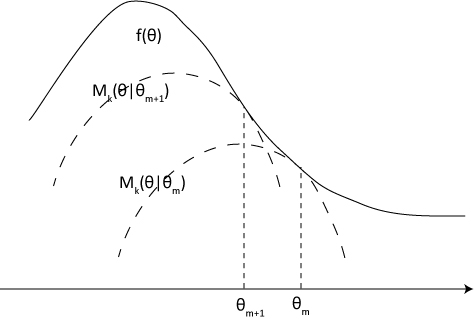
  3. 可以看成一个real-time online learning process连续的提炼best policy到一个target network,因此可以高效的记录$Q$-learning policy的进化过程。

所有的contributions可以总结为:

  1. single game distillation
  2. single game distillation with highly compressed models
  3. multi-game distillation
  4. online distillation

Single Task Policy Distillation

Distillation将teacher model T的knowledge进行迁移,得到一个参数更少更加高效的student model S。分类网络中distillation的目标通常是将teacher network layer的最后一层传入softmax layer,使用回归学习student model S的参数。
而本节介绍的single task policy distillation,是对$Q$函数而不是对classifier进行transfer,会面临以下问题:

  • 一方面,Q是unbounded and unstable,所以它的scale很难确定。此外,计算一个fixed policy的Q值需要很大的计算量。
  • 另一方面,让S只预测一个single best action也可能会出现问题,可能有很多actions的Q值接近。

给定teach model T,用它生成大小为$N$的样本集合$D^T = \left[(s_i, \mathbf{q}_i)\right]_{i=0}^T $,每一个样本是$s_i$和$\mathbf{q}_i$,$s_i$是一个observation,$\mathbf{q}_i$是对应$s_i$处每一个action的$q$值向量。
作者给出了三种policy distillation方法。如下所示:

Negative log likelyhood loss (NLL)

第一种方法使用teacher中具有最大$Q$值的action $a_{i,best} = \arg\max(\mathbf{q}_i$,使用负的log似然loss训练student model $S$直接预测action:
$$L_{NLL} (D^T, \theta_{S}) = - \sum_{i=1}^{\vert D\vert} \log P(a_i=a_{i,best} | x_i, \theta_S)\tag{1}$$

Mean squared error loss (MSE)

第二种方法计算S和T中$Q$值的mse loss:
$$L_{MSE} (D^T, \theta_{S}) = - \sum_{i=1}^{\vert D\vert} || \mathbf{q}_i^T - \mathbf{q}_i^S ||^2_2 \tag{2}$$
这种方法在student model中保留每个action的所有$Q$值。

KL divergence

第三种方法将$Q$值输入softmax layer,相当于求了policy,然后计算S和T的KL散度:
$$L_{KL} (D^T, \theta_{S}) = - \sum_{i=1}^{\vert D\vert} softmax(\frac{\mathbf{q}_i^T }{\tau})\log \frac{softmax(\frac{\mathbf{q}_i^T}{\tau}) }{softmax(\mathbf{q}_i^T) }\tag{3}$$
在传统的分类问题中,$\mathbf{q}^T $的输出是一个peaked distribution,可以通过提高softmax的温度进行soften将更多的信息transfer到student model。
而在policy distillation中,teacher的输出不是一个distribution,而是每个state下所有可能actions的$q$值,我们的目的不是soften它们,而是想要让它们更sharper。
这个和actor-mimic中的policy regressive objective是不是一样。

Multi-Task Policy Distillation

上面介绍的是单个任务的distillation,这一节介绍multi-task distillation。multi task distillation和single task distallation的过程一样,只不过在中multi task的distillation使用$n$个单独训练完成的DQN experts,使用这$n$个task上的DQN experts distill一个student model,每一个episode切换一个task。因为不同的tasks可能有不同的action sets,每一个task都有一个单独的output layer。在multitask中使用了KL和NLL loss。
这篇文章还对比了multi-task DQN agents和multi-task distillation agents的性能,Multi task DQN是训练一个network同时玩多个游戏,但是没有DQN exoerts的指导。Multi-task DQN和single-game learning的过程类似,不断的优化网络参数,预测给定state处action的$q$值。和multi-task distillation过程一样,每一个episode切换一个task,每一个task有单独的buffer,在每一个task之间不断的交错训练,并且每一个task有单独的output layer。但是multi-task DQN agents无法达到单个DQN expert的性能。可能是因为在训练过程中,不同task之间policy,reward等的相互干扰。

Multi-task distillation和multi-task DQN之间的区别:

  • multi-task distillation使用了$n$个DQN expert,即已经训练好的在单个task上都表现不错model,使用他们distill一个新的model。
  • multi-task distillation是用一个model回归拟合$n$个model。
  • multi-task learning没有使用DQN expert,而是使用一个model去玩$n$个游戏。
  • multi-task learning 是train。

Policy distillation可能提供了一种方式将多个polices组合到一个model中而不损害performance,在distillation process中,policy被压缩并且refined了。

实验

  • single game policy distillation:
    四个游戏,四个网络:dqn expert, distill-MSE, distill-NLL,distill-KL,四个网络的大小都和nature DQN一样。
  • single game policy distillation with compression
    十个游戏,四个网络:dqn expert, $25\%$ distill-KL,$7\%$ distill-KL,$4\%$ distill-KL,后面三个网络大小分别是dqn expert的$25\%, 7\%, 4\%$。
  • multi-task distillation
    三个游戏,三个网络:multi-dqn, multi-dist-NLL, multi-dist-KL,这三个网络的大小都和nature dqn一样。
    十个游戏,一个网络:multi-dist-KL,大小是nature dqn的4倍。
  • online policy distillation:

Single game policy distillation实验中,teacher network是一个已经训练完成的model,选择一个DQN expert作为teacher network,训练student network时,teacher network不进行Q-learning,只是用来采样,相当于产生监督学习的样本。Student network学习teacher network是怎么将输入和label对应的。Teacher network的输入(images)和输出(Q值)都被存在buffer中。Multitask policy distillation的训练过程类似。
除了模型压缩时候用到的DQN,以及一个$10$个games的multi-task distillation任务中用到的DQN,它的参数比nature DQN多四倍还有额外的fully connected layer,所有其他的DQN都和nature DQN的结构一样。
评价指标用的是Double DQN中的normalized score。

single game policy distillation

在这个实验中,作者测试了single game的distillation,将一个DQN expert的knowledge迁移到一个新的结构相同的随机初始化的DQN。分别使用了三种loss:MSE, NLL,KL散度进行训练。结构证明KL好于NLL好于MSE。
原因分析:
MSE是因为$Q$值在一定范围内,MSE loss都会很小,如果某个state处不同action的Q值很接近的话,即使MSE很小,也会产生误差。
NLL loss假设每次只有一个optimal action,原则上没有错。但是我们的teacher network可能不是optimal,最小化NLL的过程可能将一些noise也进行了变化。

policy distillation with model compression

这一节介绍的是policy distillation model compression。训练的时候,模型大一些有助于训练,但是训练好的模型进行压缩也保留性能。 
分别在$10$个不同的atarti游戏上进行single-game distilled,使用的都是KL loss,student分别压缩为teacher的$25\%, 7\%, 4\%$,压缩到$25\%$ student network的平均性能是teacher network的$108\%$,压缩到$25\%$ student network的平均性能是teacher network的$102\%$, 压缩到$25\%$ student network的$4\%$的平均性能是teacher network的$84\%$。
single policy distillation with model compression中网络结构:
Agent | Input | Conv. 1 | Conv. 2 | Conv. 3 | F.C. 1 | Output | Parameters
Teacher (DQN) | 4 | 32 | 64 | 64 | 512 | up to 18 | 1,693,362
Dist-KL-net1 | 4 | 16 | 32 | 32 | 256 | up to 18 | 427,874
Dist-KL-net2 | 4 | 16 | 16 | 16 | 128 | up to 18 | 113,346
Dist-KL-net3 | 4 | 16 | 16 | 16 | 64 | up to 18 | 61,954
模型压缩只改变了参数的数量,没有改变模型架构。

multi-game policy distillation

Multi-task DQN是multi-task distillation的baseline,实验使用了三个游戏,multi-task DQN和单个DQN的训练过程一样,但是使用了三个游戏的experient进行训练。对比了multi task DQN,multi distillation NLL,multi distillation KL,他们的网络大小都是一样的。
最后作者还将$10$个游戏distill到一个single student network中,这个network大小是nature DQN的四倍。
multi-task distilltaion experiments中网络结构:
Agent | Input | Conv. 1 | Conv. 2 | Conv. 3 | F.C. 1 | F.C. 2 | Output | Parameters
One Teacher (DQN) | 4 | 32 | 64 | 64 | 512 | n/a | up to 18 | 1,693,362
Multi-DQN/Dist (3 games) | 4 | 32 | 64 | 64 | 512 | 128 (x3) | up to 18 (x3) | 1,882,668
Multi-Dist-KL (10 games) | 4 | 64 | 64 | 64 | 1500 | 128 (x10) | up to 18 (x10) | 6,756,721

online policy distillation

Experimental Details

Policy Distillation Training Data collection

Policy distillation online data collection和nature DQN中agent evaluation一样,DQN随机执行最多$30$个null-ops初始化episode,使用$\epsilon$-greedy($\epsilon=0.05$)算法进行$30$分钟即$108000$frames的evaluation。
DQN expert的输入是图像,输出是$Q$值,replay buffer记录$10$个小时的experience($15$Hz下共$54000$个control steps),

Distillation Targets

Agent Evaluation

使用human starts,使用$\epsilon$-greedy($\epsilon=0.05$)算法进行$30$分钟即$108000$frames的evaluation。
在multitask中,使用$\frac{\text{student score}}{\text{DQN score}}$当做metric。

代码

官方没有放出代码,有其他人的复现版本:
https://github.com/ciwang/policydistillation

参考文献

1.https://arxiv.org/pdf/1511.06295.pdf

python ptan

发表于 2019-10-12 | 更新于 2019-10-28 | 分类于 python

PyTorch Agent Net library

简介

Ptan是一个简化RL的库,它主要目标是实现两个问题的平衡:

  1. 导入库函数,只需要一行命令,就像OpenAI的baselines一样
  2. 从头开始实现

我们既不想一行命令直接调包,也不想从头开始实现一切。

模块

  • Agent:
  • ActionSelector
  • ExperienceSource
  • ExperienceSourceBuffer
  • others

Action Selector

简介

将network的输出转换成具体的action。常用的有

  • Argmax:用于使用Q网络的方法,生成离散action。
  • Policy-based:网络输出logits或者normalizaed distribution,从这个distribution中采样。

Action Selector被Agent使用,常用的有:

  • ArgmaxActionSelector
  • EpsilonGreedyActionSector
  • ProbabilityActionSelector

基类

ActionSelector

1
2
class ActionSelector:
def __call__(self, scores)

子类

ArgmaxActionSelector

1
2
class ArgmaxActionSelector(ActionSelector):
def __call__(self, scores)

EpsilonGreedyActionSector

1
2
3
class EpsilonGreedyActionSector(ActionSelector):
def __init__(self, epsilon=0.05, selector=None)
def __call(self, scores)

ProbabilityActionSelector

1
2
class ProbabilityActionSelector(ActionSelector):
def __call__(self, probs)

对比三个ActionSelector

两个GreedySelector:Argmax和EpsilonGreedy,输入都需要是q值,输出是action。
而Probability需要的输入是概率,输出是动作。

其他

EpsilonTraker

用来记录epsilon的变化。

Agent

将observation转换为actions,常见的三种方法如下:

  • Q-function:预测当前observation下所有可能采取的action的$Q$值,选择$\arg \max Q(s)$作为action。
  • Policy-based:预测$\pi(s)$的概率分布,从分布中采样。
  • Continuous Contrl:预测连续控制参数$\mu(s)$,直接输出action。

基类

BaseAgent

1
2
3
4
5
6
7
8
9
10
class BaseAgent:
# 1.
def __initial_state(self)
# 2.
def __call__(self, states, agent_states)
"""
:param states: env states list
:param agent_states: agent state list
:return: actions tuple, agent_states
"""

子类

DQNAgent

1
2
3
4
5
class DQNAgent(BaseAgent):
# 1.
def __init__(self, dqn_model, action_selector, device="cpu", preprocessor=default_states_preprocessor)
# 2
def __call__(self, states, agent_states=None)

PolicyAgent

输入的model产生离散动作的policy distribution,Policy distribution可以是logtis或者normalized distribution。
PolicyAgent调用probability action selector对这个distribution进行采样 。PolicyAgent其实就是将model和action selector组装在了一起。

1
2
3
4
5
6
class PolicyAgent(BaseAgent):
# 1.
def __init__(self, model, action_selector=actions.ProbabilityActionSelector(), device="cpu", apply_softmax=False, preprocessor=default_states_preprocessor)
# 2.
@torch.no_grad()
def __call__(self, states, agent_states=None)

ActorCriticAgent

1
2
3
4
5
class ActorCriticAgent
# 1.
def __init__(self, model, action_selector=actions.ProbabilityActionSelector(), device="cpu", apply_softmax=False, preprocessor=default_states_preprocessor)
# 2.
def __call__(self, states, agent_states=None)

其他

default_states_preprocessor

1
2
3
4
5
6
7
8
9
10
11
def default_states_preprocessor(states):
"""
Convert list of states into the form suitable for model. By default we assume Variable
:param states: list of numpy arrays with states
:return: Variable
"""
if len(states) == 1:
np_states = np.expand_dims(states[0], 0)
else:
np_states = np.array([np.array(s, copy=False) for s in states], copy=False)
return torch.tensor(np_states)

TargetNet

1
2
3
4
5
6
7
class TargetNet
# 1.
def __init__(self, model)
# 2.
def sync(self)
# 3.
def alpha_sync(self, alpha)

Experience Source

Agent不断的和env进行交互产生一系列的trajectories,Experience可以将这些交互存储起来,重复利用。Experience的主要作用有:

  1. 支持batch,利用GPU的并行计算提高训练效率
  2. 可以对transitions或者trajectory进行预处理。比如n-step DQN。
  3. ???

常见的ExperienceSource有:

  • ExperienceSource
  • ExperienceSourceFirstLast
  • ExperienceSourceRollouts
  • ExperienceReplayBuffer: :DQN中几乎不会使用刚刚获得的experience samples,因为他们是高度相关的,让训练很不稳定。Buffer用来存放experience pieces,从buffer中采样进行训练,因为buffer容量有限,老样本会被从replay buffer中删掉
  • PrioReplayBufferNaive: Complexity of sampling is O(n)
  • PrioritizedReplayBuffer: O(log(n)) sampling complexity.

基类

ExperienceSource

1
2
3
4
5
6
7
8
9
10
11
12
13
14
15
16
17
18
19
20
21
22
23
class ExperienceSource 
"""
简单的n-step source for single or multiple envs
每一个experience都有n个Experience entries的list
"""
# 1.
def __init__(self, env, agent, steps_count=2, steps_delta=1, vectorized=False)
"""
env: 环境或者list of环境
agent: 将observation 转换为actions
steps_count: 每一个experience chain的计数
steps_delta: experience items之间相隔多少个steps
vectorized: bool,OpenAI vectorized
"""
# 2.
def __iter__(self):
"""
重写for循环的iter方法
"""
# 3.返回rewards,然后重置
def pop_total_rewards(self)
# 4.返回rewards和steps,然后重置
def pop_rewards_steps(self)

ExperienceReplayBuffer

1
2
3
4
5
6
7
8
9
10
11
12
13
14
15
16
17
18
class ExperienceReplayBuffer
#
def __init__(self, experience_source, buffer_size)

#
def __len__(self)

#
def __iter__(self)

# 从experience中随机采样一个batch_size大小的样本
def sample(self, batch_size)

# 添加一个sample,类内函数
def _add(self, sample)

# 从experience_source中获得samples_numbers个样本,将其添加到buffer
def populate(self, samples_numbers)

BatchPreprocessor

1
class BatchPreprocessor

子类

ExperienceSourceFirstLast

1
2
3
4
5
6
# Q(st, at) = rt+1 + \gamma r_t+2 + ... \gamma^t+n-1 r_t+n + Q(s t+n, s t+n)
class ExperienceSourceFirstLast(ExperienceSource):
#
def __init__(self, env, agent, gamma, steps_count=1, steps_delta=1, vectorized=False)
#
def __iter(self)

PrioritizedReplayBuffer

1
2
3
4
5
6
7
8
9
10
11
class PrioritizedReplayBuffer(ExperienceReplayBuffer)
# 1.
def __init__(self, experience_source, buffer_size, alpha)
# 2.
def _add(self, *args, **kwargs)
# 3.
def _sample_proprotional(self, batch_size)
# 4.
def sample(self, batch_size, beta)
# 5.
def update_priorities(self, idxes, priorities)

QLearningPreprocessor

1
class QLearningPreprocessor(BatchPreprocessor)

其他

ExperienceSourceRollouts

1
2
3
4
5
6
7
8
9
class ExperienceSourceRollouts:
#
def __init__(self, env, agent, gamma, setps_count=5)
#
def __iter__(self)
#
def pop_total_rewards(self)
#
def pop_rewards_steps(self)

ExperienceSourceBuffer

1
class ExperienceSourceBuffer

ExperienceReplayNaive

1
class ExperienceReplayNaive

代码解析

ExperienceSource

1
2
3
4
5
6
7
8
9
10
11
12
13
14
15
16
17
18
19
20
21
22
23
24
25
26
27
28
29
30
31
32
33
34
35
36
37
38
39
40
41
42
43
44
45
46
47
48
49
50
51
52
53
54
55
56
57
58
59
60
61
62
63
64
65
66
67
68
69
70
71
72
73
74
75
76
77
78
79
80
81
82
83
84
85
86
87
88
89
90
91
92
93
94
95
96
97
98
99
100
101
102
103
104
105
106
107
108
109
110
111
112
113
114
115
116
117
118
119
120
121
122
123
124
125
126
127
128
129
130
131
132
133
134
135
136
137
138
139
140
141
142
143
144
145
146
class ExperienceSource 
"""
简单的n-step source for single or multiple envs
每一个experience都有n个Experience entries的list
"""
# 1.
def __init__(self, env, agent, steps_count=2, steps_delta=1, vectorized=False):
"""
env: 环境或者list of环境
agent: 将observation 转换为actions
steps_count: 每一个experience chain的计数
steps_delta: experience items之间相隔多少个steps
vectorized: bool,OpenAI vectorized
"""
assert isinstance(env, (gym.Env, list, tuple))
assert isinstance(agent, BaseAgent)
assert isinstance(steps_count, int)
assert steps_count >= 1
assert isinstance(vectorized, bool)
# self.pool存放envs list,类型是list
if isinstance(env, (list, tuple)):
self.pool = env
else:
self.pool = [env]
self.agent = agent
self.steps_count = steps_count
self.steps_delta = steps_delta
self.total_rewards = []
self.total_steps = []
self.vectorized = vectorized

# 2.
def __iter__(self):
# states记录所有env的所有obs
# agent_states记录
# histories记录当前的steps_count个experience
# cur_rewards记录当前episode的rewards
# cur_steps记录当前episode的steps
states, agent_states, histories, cur_rewards, cur_steps = [], [], [], [], []

# env个数, 记录每个env observation的shape,如果向量化,[>=1, >=1, ...],如果不向量化[1, 1, 1,...],不管是否向量化,长度都等于envs个数的list,
env_lens = []

# 对每一个env进行操作,生成需要记录变量的维度
for env in self.pool:
obs = env.reset()
# if the environment is vectorized, all it's output is lists of results.
# 生成state的维度
# 如果向量化obs,states的维度大于等于env数,否则states的维度和env数量一样
if self.vectorized:
obs_len = len(obs)
states.extend(obs)
else:
obs_len = 1
states.append(obs)

# [env1_obs_len, env_2_obs_len, ..., envn_obs_len]
env_lens.append(obs_len)

# 生成histories, cur_rewards,cur_steps,agent_states的维度
for _ in range(obs_len):
# 记录所有env中所有的obs
histories.append(deque(maxlen=self.steps_count))
cur_rewards.append(0.0)
cur_steps.append(0)
agent_states.append(self.agent.initial_state())

# 总的迭代次数,用于steps_delta
iter_idx = 0
# ================================分界线===========================
# 上面是iteration的初始化,生成各类信息(states, agent_states, histories)的初始值。
# 下面开始iteration
while True:
# 1.根据states生成len(states)个action
# states >= len(envs_len) 个数
actions = [None] * len(states)
states_input = []
states_indices = []
for idx, state in enumerate(states):
if state is None:
actions[idx] = self.pool[0].action_space.sample() # assume that all envs are from the same family
else:
states_input.append(state)
states_indices.append(idx)
if states_input:
states_actions, new_agent_states = self.agent(states_input, agent_states)
for idx, action in enumerate(states_actions):
g_idx = states_indices[idx]
actions[g_idx] = action
agent_states[g_idx] = new_agent_states[idx]
# 根据env_lens将actions进行合并,长度和envs number一样
grouped_actions = _group_list(actions, env_lens)

# 2.step执行action
# global_of是全局offset,相当于每个env obs初始位置,ofs是每个env的len(action_n)个维度。
global_ofs = 0

# 分别对每个env执行相应的action_n个动作
for env_idx, (env, action_n) in enumerate(zip(self.pool, grouped_actions)):
if self.vectorized:
next_state_n, r_n, is_done_n, _ = env.step(action_n)
else:
next_state, r, is_done, _ = env.step(action_n[0])
next_state_n, r_n, is_done_n = [next_state], [r], [is_done]

# ofs是每个env的局部offset
for ofs, (action, next_state, r, is_done) in enumerate(zip(action_n, next_state_n, r_n, is_done_n)):
idx = global_ofs + ofs
state = states[idx]
history = histories[idx]

cur_rewards[idx] += r
cur_steps[idx] += 1
if state is not None:
# 记录state, action, reward, done,没有记录next_state,使用完之后,更新state[idx] = next_state
history.append(Experience(state=state, action=action, reward=r, done=is_done))
# 每一个env在enumerate时都会算一次
if len(history) == self.steps_count and iter_idx % self.steps_delta == 0:
yield tuple(history)
# 更新下一步,states[idx] = next_state
states[idx] = next_state
if is_done:
# in case of very short episode (shorter than our steps count), send gathered history
if 0 < len(history) < self.steps_count:
yield tuple(history)
# generate tail of history
while len(history) > 1:
history.popleft()
yield tuple(history)
self.total_rewards.append(cur_rewards[idx])
self.total_steps.append(cur_steps[idx])
cur_rewards[idx] = 0.0
cur_steps[idx] = 0
# vectorized envs are reset automatically
states[idx] = env.reset() if not self.vectorized else None
agent_states[idx] = self.agent.initial_state()
history.clear()
global_ofs += len(action_n)
iter_idx += 1
"""
重写for循环的iter方法
"""
# 3. 重置total_rewards
def pop_total_rewards(self)
# 4. 重置total rewards和total steps
def pop_rewards_steps(self)

ExperienceSourceFirstLast

1
2
3
4
5
6
7
8
9
10
11
12
13
14
15
16
17
18
19
20
21
22
23
24
class ExperienceSourceFirstLast(ExperienceSource):
"""
def __init__(self, env, agent, gamma, steps_count=1, steps_delta=1, vectorized=False):
assert isinstance(gamma, float)
super(ExperienceSourceFirstLast, self).__init__(env, agent, steps_count+1, steps_delta, vectorized=vectorized)
self.gamma = gamma
self.steps = steps_count

def __iter__(self):
# 并不保留中间n步的experience,因为没必要,只留第一步和最后一步,中间计算rewards就行了
for exp in super(ExperienceSourceFirstLast, self).__iter__():
if exp[-1].done and len(exp) <= self.steps:
last_state = None
elems = exp
else:
last_state = exp[-1].state
elems = exp[:-1]
total_reward = 0.0
# 计算中间的rewards
for e in reversed(elems):
total_reward *= self.gamma
total_reward += e.reward
yield ExperienceFirstLast(state=exp[0].state, action=exp[0].action,
reward=total_reward, last_state=last_state)

ExperienceReplayBuffer

1
class ExperienceReplayBuffer

参考文献

1.https://github.com/Shmuma/ptan/blob/master/docs/intro.ipynb

python iteration-iterable and iterator

发表于 2019-10-12 | 更新于 2019-12-17 | 分类于 python

Iteration

Iteration并不是一个具体的东西,它是一个抽象的名词,指的是一个接一个的取某个对象的每一个项。包含隐式的,显式的loop,即while,do, for等,这叫iteration。

Iterable和iterator

而在python中,有iterator和iterable。
一个iterable object是实现了__iter__方法的object或者定义了__getitem__方法。一个iteratable object是一个可以得到iterator的object,但是它自己并不一定是iterator object。
而iterator是一个实现了__next__和__iter__方法的object。
iterable object不一定是iterator,iterator一定是iterable object。
可以使用for循环的都是ieterable object,比如str,list,但是它们不是itertor,可以使用iter()方法得到iterator
可以next()的都是iterator

iter和__iter__

所有实现了__iter__方法的object,都是iterable object,可以通过iter()方法产生iterator object。
具体示例

1
2
3
4
5
6
7
8
9
10
11
12
13
14
15
16
17
18
19
20
21
22
23
24
25
26
27
from collections import Iterator
from collections import Iterable

class Fibs:
def __init__(self, a, b):
self.a = a
self.b = b

def __iter__(self):
a = self.a
b = self.b
while True:
yield a
a, b = b, a + b

real_fibs = Fibs(0,1)

print("real_fibs is iterator? ", isinstance(real_fibs, Iterator))
print("real_fibs is iterable? ", isinstance(real_fibs, Iterable))
print("iter(real_fibs) is iterator? ", isinstance(iter(real_fibs), Iterator))
print("iter(real_fibs) is iterable? ", isinstance(iter(real_fibs), Iterable))


for idx, i in enumerate(real_fibs):
print(i)
if idx > 10:
break

其中出现了yield关键字。yield关键字的作用是每次迭代执行到该行代码时,就返回一个值,并且记住相应的位置,在下次迭代时继续从该行位置开始执行。

next和__next__

代码示例

1
2
3
4
5
6
7
8
9
10
11
12
13
14
15
16
17
18
19
20
21
22
from collections import Iterator

class A:
def __init__(self, max_v=5):
self.max_v = max_v
self.v = 0

def __iter__(self):
return self

def __next__(self):
# if self.v <= self.nax_v
self.v += 1
return self.v


if __name__ == "__main__":
a = A()
for idx, v in enumerate(a):
print(idx, v)
if (idx >= 10):
break

参考文献

1.https://stackoverflow.com/questions/9884132/what-exactly-are-iterator-iterable-and-iteration
2.https://stackoverflow.com/a/46411740/8939281
3.https://www.jianshu.com/p/f9b547874a14
4.https://www.jianshu.com/p/1b0686bc166d

gym wrappers and monitors

发表于 2019-10-09 | 更新于 2019-10-21 | 分类于 强化学习

这一篇文章主要介绍wrappers和monitors。

什么是Wrappers

对已有的environments的功能进行扩展。比如保留过去的N个observation或者对输入进行cropped。Gym提供了这样的借口,叫做Wrapper class。
Wrapper继承自Env class,构造函数只接收一个参数,要被"wrapped"的Env实例。为了添加新的逻辑,需要重写step()或者reset()方法,但是需要调用父类的original方法。为了更细粒度的满足要求,gym还提供了三个Wrapper的subclass,ObservationWrapper,RewardWrapper和ActionWrapper分别只对observation,reward和action进行重定义。他们之间的关系如下所示:
gym_wrapper
Env是一个abstract class,具体的environments如Breakout继承了Env class,实现了step(),reset()等abstract function。Wrapper继承了env class,对step(), reset()等方法进行了重载。ActionWrapper对Wrapper进行了重载,对step和reset进行了重载。
Env

  • abstract step(self, action)
  • abstract reset(self)

Breakout(Env)

  • overwrite step(self, action)
  • overwrite reset(self)

Wrapper(Env)

  • __init__(self, env): self.env = env # instance of gym environment
  • overwrite step(self, action): self.env.step(action) # 调用的是传入参数env的step函数
  • overwrite reset(self) # 调用的是传入参数env的reset函数

ActionWrapper(Wrapper)

  • overwrite step(self, action): self.env.step(self.action(action)) # 调用的是self.env的step函数
  • overwrite reset(self) # 调用的是self.env的step函数
  • abstract action(self, action)
  • abstract reverse_action(self, action)

MyownActionWrapper(ActionWrapper)

  • overwrite action(self, action)

Wrapper示例

1
2
3
4
5
6
7
8
9
10
11
12
13
14
15
16
17
18
19
20
21
22
23
24
25
26
27
28
29
30
31
32
33
34
35
36
37
38
39
40
41
42
43
44
45
46
import gym
import random
import time


class RandomActionWrapper(gym.ActionWrapper):
def __init__(self, environment, epsilon=-1.1):
super(RandomActionWrapper, self).__init__(environment)
self.epsilon = epsilon

def action(self, action):
if random.random() < self.epsilon:
print("Random")
return self.env.action_space.sample()
# return self.environment.action_space.sample()
else:
# print("Not random")
pass
return action

def reverse_action(self, action):
pass


if __name__ == "__main__":
environment = gym.make("CartPole-v0")
env = RandomActionWrapper(environment)

obs = env.reset()
episode = 0
total_steps = 0
total_reward = 0
while True:
action = env.action_space.sample()
obs, reward, done, info = env.step(action)
print(reward)
total_reward += reward
total_steps += 1
env.render()
time.sleep(0.1)
if done:
print("Episode %d done in %d steps, total reward %.1f" %(episode, total_steps, total_reward))
time.sleep(0.1)
env.reset()
episode += 1
total_reward = 0

在这个例子中,env其实是RandomActionWrapper的对象,而RandomActionWrapper继承自ActionWrapper,对ActionWrapper的action方法进行了重载。这个Wrapper对象拥有CartPole environment的对象,调用wrapper对象的step方法时,其实调用的是ActionWrapper的step方法,而ActionWrapper调用的是self.env.env(self.action(action))。
最终其实就是将env.step(action)改成了env.step(action(action))。

什么是Monitors

使用gym.wrapper.Monior记录当前agent的执行动作。它的使用方法很简单,如下所示:

1
2
env = gym.make("CartPole-v0")
env = gym.wrappers.Monitor(env, "path")

只需要在env的外面套上一个Monitor即可,它会自动记录玩游戏的过程。

Wrapper in baselines

Openai baselines中实现了许多wrappers。它们包括:

  • 将一个大的episode切分成更小的episode,一个游戏可能有好几条命,原来的实现中是这几条命都是一个episode,现在把它改成一条命一个episode
  • 执行至多$30$个no-op。
  • frame-skip和取最后两帧中pixel更大的那个当做observation
  • 在游戏开始时Pressing FIRE,一般在重置游戏的时候,有些游戏需要按一下fire才会开始,否则一直都是fixed。
  • Image cropped,将$210\times 160$三通道转换成$84\times 84$单通道
  • Stacking $4$ frames当做observation
  • Clipped reward 到$-1, 0, 1$,或者$[-1, 1]$
  • 将$0-255$之间的值转换成$[0.0, 1.0]$

Monitors示例

1
2
3
4
5
6
7
8
9
10
11
12
13
14
15
16
17
18
19
20
21
22
23
24
25
import gym
import time

if __name__ == "__main__":
env = gym.make("CartPole-v0")
env = gym.wrappers.Monitor(env, "recording")

total_reward = 0.0
total_steps = 0
obs = env.reset()
episode = 1
while True:
action = env.action_space.sample()
obs, reward, done, _ = env.step(action)
total_reward += reward
total_steps += 1
env.render()
if done:
print("Episode %d done in %d steps, total reward %.2f" %(episode, total_steps, total_reward))
time.sleep(1)
env.reset()
if episode > 5:
break
episode += 1
total_reward = 0

参考文献

1.https://hub.packtpub.com/openai-gym-environments-wrappers-and-monitors-tutorial/
2.https://www.packtpub.com/big-data-and-business-intelligence/deep-reinforcement-learning-hands
3.https://discuss.pytorch.org/t/in-the-official-q-learning-example-what-does-the-env-unwrapped-do-exactly/28695/2

python pickle

发表于 2019-10-08 | 更新于 2019-12-17 | 分类于 python

简介

pickle是一个序列化模块,它能将python对象序列化转换成二进制串再反序列化成python对象。

常用函数

pickle.dump()

API

1
pickle.dump(obj, file, [,protocol])

作用

将python对象obj以二进制字符串形式保存到文件file中,使用protocol。

示例

1
2
3
4
5
6
import pickle

dictionary = {"name": "mxx", "age": 23}

with open("test.txt", 'wb') as f:
pickle.dump(dictionary, f)

pickle.load()

API

1
pickle.load(file)

作用

从文件file中读取二进制字符串,将其反序列成python对象。

示例

1
2
3
4
5
6
7
import pickle

with open("test.txt", 'rb') as f:
b = pickle.load(f)

print(b)
print(type(b))

pickle.dumps()

API

1
pickle.dumps(obj, [,protocol])

作用

将python对象obj转化成二进制字符串,返回一个字符串

示例

1
2
3
4
5
6
7
8
9
10
import pickle

dictionary = {"name": "mxx", "age": 23}

s = pickle.dumps(dictionary)
print(s)
print(type(s))
# 输出
# b'\x80\x03}q\x00(X\x04\x00\x00\x00nameq\x01X\x03\x00\x00\x00mxxq\x02X\x03\x00\x00\x00ageq\x03K\x17u.'
# <class 'bytes'>

pickle.loads()

API

1
pickle.loads(string)

作用

从二进制字符串中返回序列化前的python obj对象。

示例

1
2
3
4
5
6
7
8
import pickle

dictionary = {"name": "mxx", "age": 23}

s = pickle.dumps(dictionary)
b = pickle.loads(s)
print(b)
print(type(b))

参考文献

1.https://www.jianshu.com/p/cf91849064e3

python mpi4py

发表于 2019-10-08 | 更新于 2019-12-17 | 分类于 python

MPI

MPI全名是Message Passing Interface,它是一个标准,而不是一个实现,专门为进程间通信实现的。它的工作原理很简单,启动一组进程,在同一个通信域中的不同进程有不同的编号,可以给不同编号的进程分配不同的任务,最终实现整个任务。
MPI4PY就是python中MPI的实现。在python中有很多种方法实现多进程以及进程间通信,比如multiprocessing,但是multiprocessing进程间通信不够方便,mpi4py的效率更高一些。
mpi4py提供了点对点通信,点对面,面对点通信。点对点通信又包含阻塞和非阻塞等等,通信的内容包含python内置对象,也包含numpy数组等。

mpi4py简单对象和方法介绍

MPI.COMM_WORLD是一个通信域,在这个通信域中有不同的进程,每个进程的编号以及进程的数量都可以通过这个通信域获得。具体看以下comm_world.py代码:

1
2
3
4
5
6
7
8
from mpi4py import MPI

# 获得多进程通信域
comm = MPI.COMM_WORLD
# 获得当前进程通信域中进程数量
size = comm.Get_size()
# 获得当前进程在通信域中的编号
rank = comm.Get_rank()

mpiexec -np 3 python comm_world.py

点对点通信

阻塞通信

python对象

简介

comm.send(data, dest, tag)
comm.recv(source, tag)
send和recv都是阻塞方法,即调用这个方法之后,等到该函数调用结束之后再返回。dest是目的process编号,source是发送的process编号。data是要发送的数据,需要是python的内置对象,即可以pickle的对象。

代码示例
1
2
3
4
5
6
7
8
9
10
11
12
13
from mpi4py import MPI

comm = MPI.COMM_WORLD
rank = comm.Get_rank()
size = comm.Get_size()

if rank == 0:
data = {'name': "mxx", "age": 23}
comm.send(data, dest=1, tag=10)
print("data has sent.")
else:
data = comm.recv(source=0, tag=10)
print("data has been receieved.")

numpy数组

简介

comm.Send(data, dest, tag)
comm.Recv(source, tag)
Send和Recv都是阻塞方法,即调用这个方法之后,等到该函数调用结束之后再返回。dest是目的process编号,source是发送的process编号。data是要发送的数据,需要是numpy对象,和c语言的效率差不多。

代码示例
1
2
3
4
5
6
7
8
9
10
11
12
13
14
from mpi4py import MPI

comm = MPI.COMM_WORLD

rank = comm.Get_rank()
size = comm.Get_size()

if rank == 0:
data = {'name': "mxx", "age": 23}
comm.isend(data, dest=1, tag=10)
print("data has sent.")
else:
data = comm.irecv(source=0, tag=10)
print("data has been receieved.")

非阻塞通信

简介

comm.isend(data, dest, tag)
comm.irecv(source, tag)
isend和irecv都是非阻塞方法,即调用这个方法之后,调用该函数之后立即返回,无需等待它执行结束。dest是目的process编号,source是发送的process编号。data要是python对象,可以被pickle处理的。

代码示例

1
2
3
4
5
6
7
8
9
10
11
12
13
14
15
16
17
from mpi4py import MPI
import numpy as np

comm = MPI.COMM_WORLD

rank = comm.Get_rank()
size = comm.Get_size()


if rank == 0:
data = np.ones((3, 4), dtype='i')
comm.Send([data, MPI.INT], dest=1, tag=10)
print("data has sent.")
else:
data = np.empty((3, 4), dtype='i')
data = comm.Recv([data, MPI.INT], source=0, tag=10)
print("data has been receieved.")

组通信

bcast

简介

将一个process中的数据发送给所有在通信池中的process。
comm.bcast(data, dest, tag)

代码示例

1
2
3
4
5
6
7
8
9
10
11
12
13
14
15
import mpi4py
from mpi4py import MPI

comm = MPI.COMM_WORLD
size = comm.Get_size()
rank = comm.Get_rank()

if rank == 1:
data = {"name": "mxx", "age": 23}
print("data bcast to others")
else:
data = None

data = comm.bcast(data, root=1)
print("process {} has received data".format(rank))

scatter

简介

将一个process的数据拆分成n份,发送给所有在通信池中的process每个一份,和bcast的区别在于,bcast发送的数据对于每一个process都是一样的,而scatter是将一份数据拆分成n份分别发送给每个process。
comm.scatter(data, dest, tag)

代码示例

1
2
3
4
5
6
7
8
9
10
11
12
13
14
15
16
import mpi4py
from mpi4py import MPI

comm = MPI.COMM_WORLD
size = comm.Get_size()
rank = comm.Get_rank()

recv_data = None
if rank == 1:
send_data = range(size)
print("data bcast to others")
else:
send_data = None

recv_data = comm.scatter(send_data, root=1)
print("process {} has received data {}".format(rank, recv_data))

gather

简介

和comm.bcast相反,将每个process中的数据收集到一个process中。
comm.gather(data, dest, tag)

代码示例

1
2
3
4
5
6
7
8
9
10
11
12
13
14
import mpi4py
from mpi4py import MPI


comm = MPI.COMM_WORLD
size = comm.Get_size()
rank = comm.Get_rank()

send_data = rank
print("process {} send data {} to root.".format(rank, send_data))

recv_data = comm.gather(send_data, root=9)
if rank == 9:
print("process {} gather all data {} to others.".format(rank, recv_data))

参考文献

1.https://zhuanlan.zhihu.com/p/25332041
2.https://www.jianshu.com/p/f497f3a5855f

gradient method deep deterministic policy gradient

发表于 2019-10-06 | 更新于 2019-12-17 | 分类于 强化学习

ddpg

论文名称:CONTINUOUS CONTROL WITH DEEP REINFORCEMENT LEARNING
论文地址:https://arxiv.org/pdf/1509.02971.pdf

摘要

本文将DQN的思路推广到continuous action domain上。DQN是离散空间,DDPG是连续空间。

简介

强化学习的目标是学习一个policy最大化$J=\mathbb{E}_{r_i,s_i\sim E, a_i\sim \pi}\left[R_1\right]$的expected return。
简要回顾以下action-value的定义,它的定义是从状态s开始,采取action a,采取策略$\pi$得到的回报的期望。
$$Q{\pi}(s_t,a_t) = \mathbb{E}_{r_{i\ge t}, s_{i \gt t}\sim E,a_{i\gt t}\sim \pi}\left[R_t|s_t,a_t\right] \tag{1}$$
(注意,这里$R$的下标和reinforcement learning an introduction中的定义不一样,但是这个无所谓,只要在用的时候保持统一就好了。)
许多rl方法使用bellman方程递归的更新Q:
$$Q{\pi}(s_t,a_t) = \mathbb{E}_{r_t,s_{t+1}\sim E}\left[r(s_t,a_t) + \gamma\mathbb{E}_{a_{t+1}\sim\pi}\left[Q^{\pi} (s_{t+1},a_{t+1})\right]\right]\tag{2}$$
如果target policy是deterministic的话,用$\mu$表示,那么就可以去掉式子里面的期望,action是deterministic的而不是服从一个概率分布:
$$Q{\mu}(s_t,a_t) = \mathbb{E}_{r_t,s_{t+1}\sim E}\left[r(s_t,a_t) + \gamma Q^{\mu} (s_{t+1},\mu(s_{t+1}))\right] \tag{3}$$
而第一个期望只和environment相关。这就意味着可以使用off-policy方法学习$Q{\mu}$。
在DQN中,作者使用replay buffer和target network缓解了non-linear funnction approximator不稳定的问题,作者在这篇文章将它们推广到了DDPG上面。

DDPG

直接将Q-learning推广到continuous action space是不可行的,因为action是continuous的,对其进行max等greedy操作是不可行的。这种优化方法只适合trival action spaces的情况。所以这里使用的是DPG(deterministic policy gradient),将其推广到non-linear case,DPG是一种actor-critic的方法。
DPG使用一个参数化的actor function $\mu(s|\theta{\mu})$作为当前的policy,它将一个states直接mapping到一个specific action。$Q(s,a)$作为critic使用Q-learning中的Bellman公式进行更新。Actor的更新直接应用chain rule到$J$的expected reutrn ,更新actor的参数如下:
\begin{align*}
\nabla_{\theta{\mu}} &\approx \mathbb{E}_{s_t\sim \rho^{\beta} }\left[\nabla_{\theta^{\mu} }Q(s,a|\theta^Q )|_{s=s_t, a= \mu(s_t|\theta^{\mu} )}\right]\\
&= \mathbb{E}_{s_t\sim \rho{\beta}}\left[\frac{\partial Q(s,a|\theta^Q )}{\partial\theta^{\mu} }|_{s=s_t, a= \mu(s_t|\theta^{\mu} )}\right]\\
&= \mathbb{E}_{s_t\sim \rho{\beta}}\left[\frac{\partial Q(s,a|\theta^Q )}{\partial a}|_{s=s_t, a= \mu(s_t)}\frac{\partial \mu(s_t|\theta^{\mu} )}{\partial\theta^{\mu} }|_{s=s_t}\right]\\
&= \mathbb{E}_{s_t\sim \rho{\beta}}\left[\nabla_a Q(s,a|\theta^Q )|_{s=s_t, a= \mu(s_t)} \nabla_{\theta_{\mu}} \mu(s|\theta_{\mu})|_{s=s_t}\right]\\ \tag{4}
\end{align*}
中间的两行是我自己加的,不知道对不对,DPG论文中有证明,还没有看到,等到读完以后再说补充把。

Contributions

本文的几个改进:

  1. 使用replay buffer,
  2. 使用target network解决不稳定的问题。
  3. 使用了batch-normalization。
  4. exploration。off policy的一个优势就是target policy和behaviour policy可以不同。本文使用的behaviour policy $\mu’$ 添加了一个从noise process $N$中采样的noise:
    $$\mu(s_t) = \mu(s_t|\theta_t{\mu}) + N \tag{5}$$

算法

算法1 DDPG
随机初始化critic 网络$Q(s,a |\theta Q)$,和actor网络$\mu(s|\theta^{\mu} )$的权重$\theta^Q $和$\theta^{\mu} $
初始化target networks $Q’$和$\mu’$的权重$\theta{Q’}\leftarrow \theta^Q ,\theta^{\mu’} \leftarrow \theta^{\mu} $
初始化replay buffer $R$
for episode = 1, M do
初始化一个随机process $N$用于exploration
receive initial observation state $s_1$
for $t=1, T$ do
根据behaviour policy选择action $a_t = \mu(s_t| \theta{\mu}) + N_t$
执行action $a_t$,得到$r_t$和$s_{t+1}$
将transition $s_t, a_t, r_t, s_{t+1}$存到$R$
从$R$中采样$N$个transition $s_i, a_i, r_i, s_{i+1}$
设置target value $y_i = r_i + \gamma Q’(s_{i+1}, \mu’(s_{i+1}|\theta{\mu’})|\theta^{Q’} )$
使用$L = \frac{1}{N}\sum_i(y_i-Q(s_i,a_i|\theta Q))^2 $更新critic
使用sampled policy gradient 更新acotr:
$$\nabla_{\theta{\mu}}\approx \frac{1}{N}\sum_i\nabla_a Q(s,a|\theta^Q )|_{s=s_i, a=\mu(s_i)}\nabla_{\theta^{\mu} }\mu(s|\theta^{\mu} )|_{s_i}$$
更新target networks:
$$\theta’\leftarrow \tau \theta + (1-\tau) \theta’$$
end for
end for

实验

所有任务中,都使用了low-dimensional state和high-dimensional renderings。在DQN中,为了让问题在high dimensional environment中fully observable,使用了action repeats。在agent的每一个timestep中,进行$3$个timesteps的仿真,包含repeating action以及rendering。因此agent的observation包含$9$个feature maps(RGB,每一个有3个renderings),可以让agent推理不同frames之间的differences。frames进行下采样,得到$64\times 64$的像素矩阵,然后$8$位的RGB值转化为$[0,1]$之间的float points。
在训练的时候,周期性的进行test,test时候的不需要exploration noise。实验表明,去掉不同的组件,即contribution中的几点之后,结果都会比原来差。没有使用target network的话,结果尤其差。
作者使用了两个baselines normalized scores,第一个是naive policy,在action space中均匀的采样action得到的mean return,第二个是iLQG。normalized之后,naive policy的mean score是0,iLQG的mean score是$1$。DDPG能够学习到好的policy,在某些任务上甚至比iLQG还要好。

参考文献

1.https://arxiv.org/pdf/1509.02971.pdf

reinforcement learning why use baseline ?

发表于 2019-10-04

reinforcement learning importance sampling

发表于 2019-09-27 | 更新于 2019-12-17 | 分类于 强化学习

Importance Sampling

Importance sampling是使用一个分布近似估计另一个分布期望的方法,即通过分布$q$计算分布$p$下$f(x)$的期望。通过从$q$中采样而不是从$p$中采样近似:
$$\mathbb{E}_p\left[f(x)\right] = \mathbb{E}_q\left[ \frac{p(x)f(x)}{q(x)}\right] \tag{1}$$
使用采样分布$q$估计分布$p$下的期望:
$$\mathbb{E}_p\left[f(x)\right] \approx \frac{1}{n} \sum_{i=1}^n \frac{p(x_i)f(x_i)}{q(x_i)} x_i\sim q\tag{2}$$
上面的公式需要满足$p(x_i)$不为$0$时,$q(x_i)$也不为$0$。直接计算$\mathbb{E}_p\left[f(x)\right]$和$\mathbb{E}_q\left[f(x)\right]$,一般来说是不同的,通过importance ratio调整权重,就可以使用$q$分布估计$p$分布的期望了。举个例子:
$$f(1) = 2, f(2) = 3, f(3) = 4, otherwise 0 \tag{3}$$
概率分布$p$为:$p(x=1) = 0, p(x=2) = \frac{1}{3},p(x=3) = \frac{2}{3}$,概率分布$q$为:$q(x=1) = \frac{1}{3}, q(x=2) = \frac{1}{3}, q(x=3) = \frac{1}{3}$。计算期望,$\mathbb{E}_p\left[f(x)\right] = \frac{11}{3}$,$\mathbb{E}_q\left[f(x)\right] = 3$
使用importance ratio进行权重调整:
\begin{align*}
\mathbb{E}_p\left[f(x)\right] & = \mathbb{E}_q\left[\frac{q(x)}{p(x)}f(x)\right] \\
& = \mathbb{E}_q\left[\frac{p(x=1)}{q(x=1)}f(x=1) \right] + \mathbb{E}_q\left[\frac{p(x=2)}{q(x=2)}f(x=2) \right] + \mathbb{E}_q\left[\frac{p(x=3)}{q(x=3)}f(x=3) \right] \\
& = \frac{1}{3}*0 + \frac{1}{3}\frac{\frac{1}{3}}{\frac{1}{3}}*3 + \frac{1}{3}\frac{\frac{2}{3}}{\frac{1}{3}}*4\\
& =\frac{11}{3}\\
\end{align*}
可以看出来,我们使用分布$q$估计除了分布$p$的期望。通过使用一个简单分布$q$进行采样,可以计算出$p$的期望。在RL中,通常通过复用old policy的sample trajectory学习current policy。

Optimal Importance Sampling

Importance sampling使用采样近似估计$\mathbb{E}_p\left[f(x)\right]\approx \frac{1}{N}\sum_i \frac{p(x_i)}{q(x_i)}f(x_i)$近似计算$\mathbb{E}_p\left[f(x)\right]$。随着样本数量$N$的增加,期望值越准确。但是这种方法的方差很大,为了减少方差,样本分布$q$应该满足:
$$q(x) \propto p(x)\vert f(x)\vert \tag{4}$$
简单来说,为了减少方差,我们需要采样return更大的点。

Normalized importanct sampling

上面介绍的方法叫做unnormalized importance sampling。可以使用下里面的公式将unnormalized importance sampling转换为normalized importance sampling。
$$p(x) = \frac{\hat{p}(x)}{Z}\tag{5}$$
许多ML方法属于贝叶斯网络或者马尔科夫随机场,对于贝叶斯网络中,$p$很容易计算。但是当$p$是马尔科夫随机场时,$\sum\hat{p}(x)$是很难计算的。
\begin{align*}
\mathbb{E}_p\left[f(x)\right] & = \int f(x) p(x) dx\\
& = \int f(x) \frac{\hat{p}(x)}{Z} \frac{q(x)}{q(x)} dx\\
& = \frac{\int f(x) \hat{p}(x) \frac{q(x)}{q(x)}dx}{Z}\\
& = \frac{\int f(x) \hat{p}(x) \frac{q(x)}{q(x)} dx}{\int \hat{p}(x) dx}\\
& = \frac{\int f(x) \hat{p}(x) \frac{q(x)}{q(x)} dx}{\int \hat{p}(x)\frac{q(x)}{q(x)} dx}\\
& = \frac{\int f(x) q(x)\frac{\hat{p}(x)}{q(x)} dx}{\int q(x)\frac{\hat{p}(x)}{q(x)} dx}\\
& = \frac{\int f(x) r(x)q(x) dx}{\int r(x)q(x) dx}\qquad\qquad 记r(x) = \frac{\hat{p}(x)}{q(x)}\\
\end{align*}
接下来用采样样本的求和近似积分求期望:
\begin{align*}
\mathbb{E}_p\left[f(x)\right] & = \frac{\int f(x) r(x)q(x) dx}{\int r(x)q(x) dx}\qquad\qquad 记r(x) = \frac{\hat{p}(x)}{q(x)}\\
& \approx \frac{\sum_i f(x^i) r^i }{\sum r^i}\qquad\qquad 其中 r^i = \frac{\hat{p}(x^i ) }{q(x^i ) }\\
& = \sum_i f(x^i) r^i \frac{r^i}{\sum_i r^i}\\
\end{align*}
通过计算
这就避免了计算$Z$,这种方法叫做normalized importance sampling。但是需要付出一定代价,unnormalized importance sampling是无偏的,而normalized importance是有偏的但是方差更小。

Importance sampling in RL

我们可以使用importance sampling方法从old policy $\pi’$采样估计new policy $\pi$的值函数。计算一个action的returns的代价很高,但是如果新的action和老的action很接近,importance sampling可以帮助我们利用old calculation计算新的returns。举个例子,在MC方法中,无论何时更新$\theta$,都需要根据新的trajectories计算returns。
$$\nabla_{\theta}J(\theta) = \frac{1}{N}\sum_{i=1}^T \left(\sum_{t=1}^T \nabla_{\theta} \log \pi_{\theta}(a_{i,t}|s_{i,t})\right)\left(\prod_{t=1}^T R(s_{i,t},a_{i,t})\right) \tag{6}$$
一个trajectory可以有几百个steps,单个的更新是非常低效的。有了importance sampling之后,我们可以基于old samples计算新的return。然而,如果两个policy差的太远,accuracy会降低。因此周期性的同步policy是非常必要的。
使用importance sampling,重写policy gradient的等式:
$$\nabla_{\theta}J(\theta) = \mathbb{E}_{\tau\sim\bar{\pi}(\tau)}\left[\sum_{t=1}^T \nabla_{\theta} \log \pi_{\theta}(a_t|s_t)\left(\prod_{t’=1}^T \frac{\pi_{\theta}(a_{t’}|s_{t’})}{\hat{\pi}_{\theta}(a_{t’}|s_{t’})}\right)\left(\prod_{t’=t}^T R(s_{t’},a_{t’})\right)\right]\tag{7}$$
为了约束policy的变化,可以加入trust region约束条件,在这个region内,我们认为使用importance sampling得到的结果是可信的:
$$\max_{\theta} \hat{\mathbb{E}}_t\left[\frac{\pi_{\theta}(a_t|s_t)}{\pi_{\theta_{old}}(a_t|s_t}\hat{A}_t\right]\tag{8}$$
$$s.t. \hat{\mathbb{E}}_t\left[\text{KL}\left[\pi_{\theta_{old}}(\cdot|s_t),\pi_{\theta}(\cdot|s_t)\right]\right]\tag{9}$$

参考文献

1.https://medium.com/@jonathan_hui/rl-importance-sampling-ebfb28b4a8c6
2.http://webee.technion.ac.il/people/shimkin/MC15/MC15lect4-ImportanceSampling.pdf

mm

发表于 2019-09-25 | 更新于 2019-12-17 | 分类于 机器学习

MM

MM是一类迭代优化方法,利用函数的凸性寻找极大值或者极小值。MM是Majoriza-Minimization或者Minorize-Maximization的缩写,取决于优化目标是maximization还是minimization。MM不是一个算法,它描述了如何如构建一个优化算法。
EM算法可以看成MM算法的一个例子。但是EM算法使用到了条件期望,而MM算法中凸性和不等式是重点。

算法思路

MM算法寻找objective function的一个替代品,然后优化新的目标函数直到一个极值点。
拿minorize-maximization算法举个例子,用$f(\theta)$表示需要被maximized的目标函数,它是一个concave函数。在第$m=0,1,\cdots$步中,构建新的目标函数$g(\theta|theta_m)$满足:
$$g(\theta|\theta_m) \le f(\theta), \forall \theta \tag{1}$$
$$g(\theta_m|\theta_m) = f(\theta_m) \tag{2}$$
式子$(1)表示$g(\theta|\theta_m)$是$f(\theta)$的下界,式子$(2)$表明$f(\theta)$和$g(\theta|\theta_m)$可以取到等号。
如下图所示:
mm
接下来,通过最大化$g(\theta|\theta_m)$就可以最大化$f(\theta)$:
$$\theta_{m+1} = \arg \max_{\theta} g(\theta|\theta_m) \tag{3}$$
当$m\rightarrow \infty$时,$f(\theta_m)$就会收敛到极小值点或者鞍点。我们能够得到以下的几个关系式:
$$f(\theta_{m+1}) \ge g(\theta_{m+1}|\theta_m) \ge g(\theta_m|\theta_m)=f(\theta_m) $$

参考文献

1.https://en.wikipedia.org/wiki/MM_algorithm

1…141516…34
马晓鑫爱马荟荟

马晓鑫爱马荟荟

记录硕士三年自己的积累

337 日志
26 分类
77 标签
RSS
GitHub E-Mail
© 2022 马晓鑫爱马荟荟
由 Hexo 强力驱动 v3.8.0
|
主题 – NexT.Pisces v6.6.0